

Lyapunov exponents
What is Lyapunov exponent
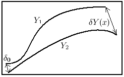
Lyapunov exponents of a dynamical system with continuous time determine the degree of divergence (or approaching) of different but close trajectories of a dynamical system at infinity. If at the beginning the distance between two different trajectories was δ0, after a rather long time x the distance would look like:
where λ - Lyapunov exponent. For different initial values the λ numbers may be different. If the corresponding Lyapunov exponent is positive, the distance between initially close trajectories of the system increases with time, if the exponent is negative - close trajectories become even closer, finally, if the exponent is zero - close trajectories remain at approximately the same distance from each other. It is known that for an N-dimensional dynamical system exist exactly N Lyapunov exponents λ1 ≥ λ2 ≥ ...≥ λN, in general, different (Oseledets Theorem, this is true for "almost all" initial states of the dynamical system). A set of Lyapunov exponents (spectrum) characterizes the general patterns of the system behavior for all possible initial conditions.
Lyapunov exponents of arbitrary dynamical systems rarely can be obtained analytically (as a formula), but there are numerical methods that allow them to be calculated with reasonable accuracy.
Lyapunov exponents are important in the qualitative theory of dynamical systems. Knowledge of Lyapunov exponents allows making a conclusion about the system behaivor over the time. Quite often it's enough to know the SIGN of the first, i.e. greatest exponent, and the TOTAL SUM of exponents.
In three dimensions, for systems of the type:
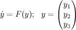
if we consider only systems that have a physical meaning, for which not all the Lyapunov exponents are positive and their sum is non-positive, and indicating by the sign "-" negative Lyapunov exponent, "+" sign is positive, and the sign "0" - zero, then the following options are available for various behavior:
-
(-,-,-) the system tends to a fixed point, i.e., to a steady state that is independent of time
-
(0,-,-) behavior of the system becomes periodic, its trajectory approaches to the closed curve (such curve is called a "limit cycle")
-
(0,0,-) quasi-periodic behavior, and the trajectories of the system are located on the surface of the two-dimensional torus, i.e. "donut"
-
(+,0,-) over the time, the system approaches the "strange attractor" (an example is the Lorenz system), the behavior of the system can be called chaotic
For systems of higher dimension the set of options becomes more numerous, but still if there is a positive Lyapunov exponent (assuming the negativity of their sum) then the system exhibits a chaotic behavior
Numerical computation of Lyapunov exponents
DEREK is able to calculate the part of the spectrum of Lyapunov exponents (not more than 4 of the first, if you place them in descending order, i.e., for systems of no more than fourth order it defines all exponents), using a numerical iterative Benettin algorithm. In this algorithm, the Lyapunov exponents are calculating using multiple solutions of the auxiliary dynamical system, which is constructed on the basis of the original. To implement this algorithm must be given an initial time step (on x ), accuracy of the solution of the system, the maximum number of iterations and the precision of Lyapunov exponents calculation. If you know that the system has zero Lyapunov exponent (this is true, for example, for an autonomous system whose trajectory does not tend to a fixed point) - you can specify the appropriate sign, this will increase the accuracy of the calculation.
DEREK can also calculate and plot the dependence of few largest Lyapunov exponents on the system parameter. To graph it user must specify the range of the parameter and the number of steps in which this range will be broken. As a result, a set of graphs is displayed showing the dependence of each of the exponent from the parameter (at points corresponding to steps). The graph can be made up of individual dots (large) and connecting lines or of both.
For Lyapunov exponents calculation using DEREK it's not required any additional software - neither compilers nor program libraries nor computer algebra packages. In addition, the user does not require any programming skills. It's simple - you must write down the equations that define the dynamical system, and then select in the graphics window menu item for Lyapunov exponents calculating, fill a form answering a few (not many) prompts (or use the default setting). After this, the user gets the numerical value of the Lyapunov exponents or plots of Lyapunov exponents dependence from system parameter.
Examples of Lyapunov exponents computation
Below it's shown the dependence of the Lyapunov exponents on the system parameter for some famous dynamical systems.
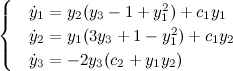
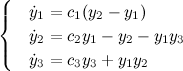
Rabinovich-Fabrikant system

Moore-Spiegel model

Lorenz model

Rössler model


When the parameter c3 is varying, at c3 ≈ 4.2 system behavior changes from periodic to chaotic, with a further increase of the parameter behavior for some values returns to the periodic.
Generator of Quasi-Periodic Oscillations
(refer to an article: V. S. Anishchenko,S. M. Nikolaev, "Generator of quasi-periodic oscillations featuring two-dimensional torus doubling bifurcations" ,or free in russian).
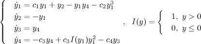
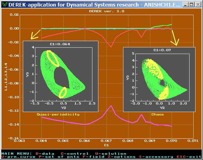
At the minimum value of the parameter the behavior of the system can be described as "quasi-periodic" (it is confirmed by the points of the Poincaré section, which located on two closed curves), at the maximum value of the parameter, the system behaves chaotically (the points of Poincaré section densely fill some areas).
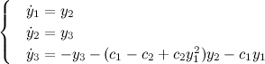
Quasi-reversible system
In an article "Shilnikov bifurcation: stationary quasi-reversal bifurcation" by Marcel G. Clerc, Pablo C. Encina and Enriquie Tirapegui following system is studied:


With c1 changing in given range the system exhibits different types of attractors. When c1 is less than 0.48,
the system's attractor is a fixed point, but not finite (the solution tends to infinity).
More information on the study of dynamical systems with the aid of the Lyapunov exponents can be learned in a "Dynamical chaos" course of lectures by S.P.Kuznetsov (in russian).

A.M. Lyapunov monument near one of the buildings of V.N. Karazin Kharkov National University